
(해당 강의노트는 Marc Peter Deisenroth, A. Aldo Faisal and Cheng Soon Ong, 『Mathematics for Machine Learning』을 기반으로 작성하였습니다)
목차
0. Introduction
1. Determinant & trace
2. Cholesky decomposition
3. Eigendecomposition: Eigenvalues & eigenvectors
4. Singular value decomposition (SVD)
0. Introduction
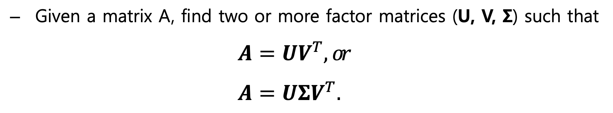
0.1 Matrix decomposition
선형대수학에서 두 방정식( A는 covariance matrix: 공분산 행렬로, 데이터를 표현)
1. linear equations, Chapter 2: $Ax = b$
2. eigenvalue equations, Chapter: Ax=λx
( x is eigen vector, λ is eigen value)
Definition
선형대수학을 시작하는 새로운 방법
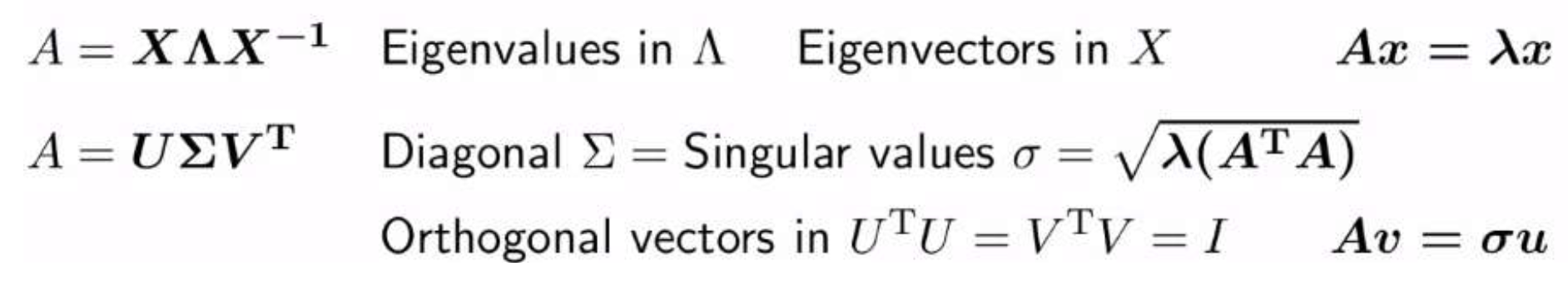
Gilbert Strang prof, in MIT : 머신러닝에서 선형대수학은 Matrix decomposition과 Linear Equation이 양대산맥이다!
아래는 이 둘의 표현 방식의 차이점
0.2 Matrix decomposition in Machine Learning
Principal component analysis (PCA)(활용 예1)

*covariance matrix란? 데이터 분포 표현으로 데이터 변수들 간의 상관관계(분산)
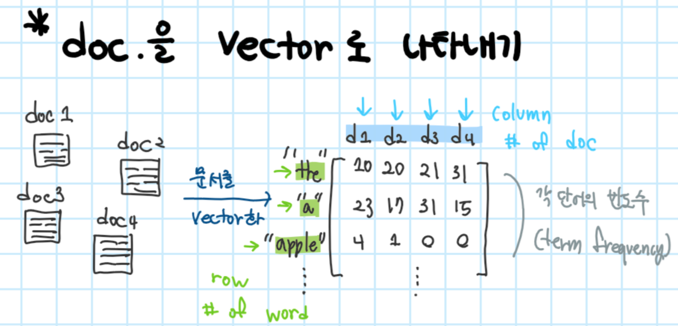
Term-document matrix(활용 예1)
- term-document matrix A : DxN (D: # of word, N : # of document)은 문서의 벡터 공간 표현의 collection이다( row(열)은 term(word)이고, column(행)은 문서에 해당)
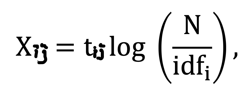
*IDF란? document frequency(DF)의 역수로 다른 문서에서 나오늘 빈도수가 높을 수록 중요도는 낮아진다. 즉 IDF는 중요도를 나타냄
*t_ij는 j번째 문서의 i번째 단어로 term frequency를 나타냄
*idf_i는 단어 i를 포함한 문서의 수임'
- 아래와 같이 표현 할 수 있음
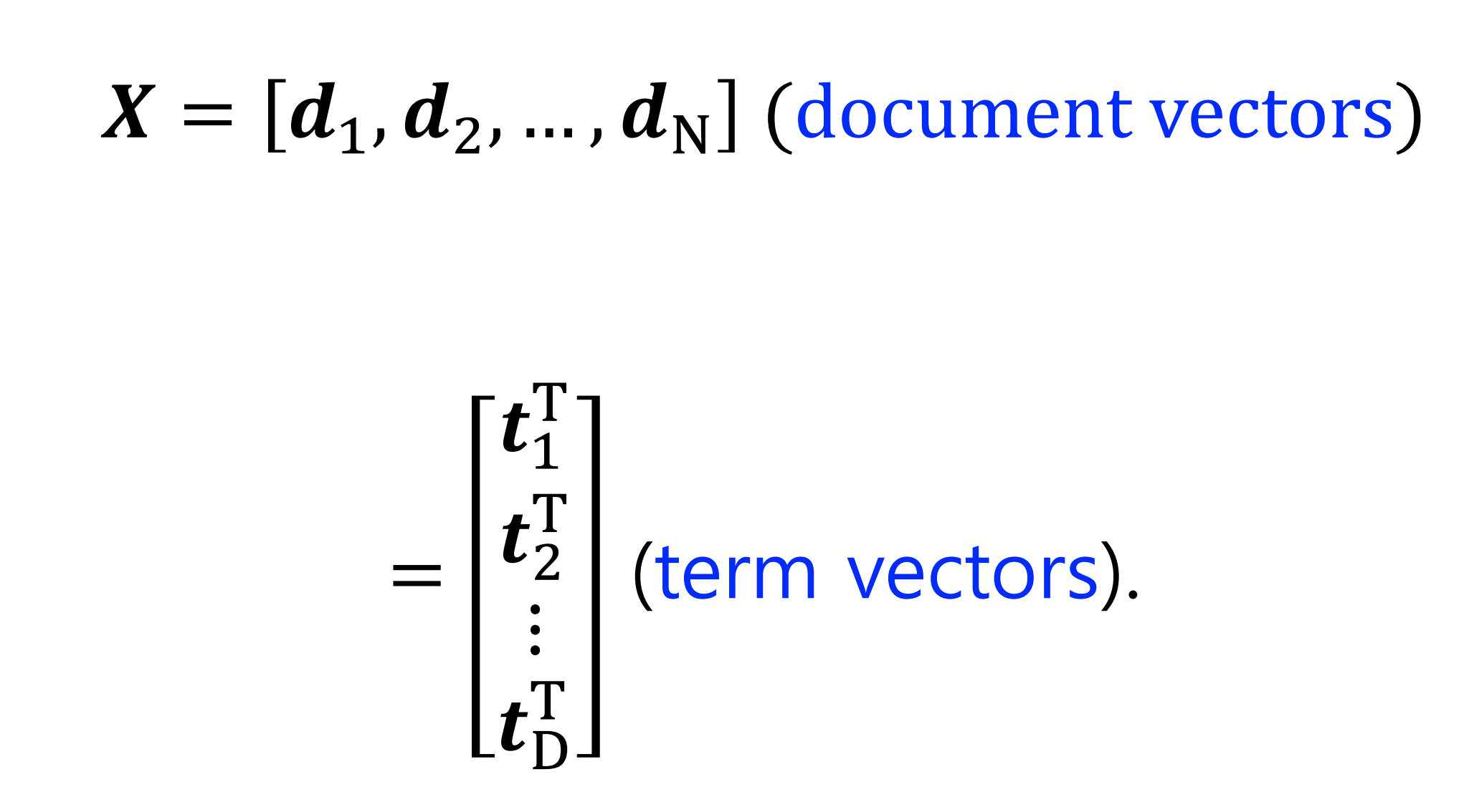
- document vector는 DxN 고차원이므로, matrix decomposition을 사용하여 low-dimensional projection을 해야 함
- Latent Semantic Analysis(LSA)
: 기본적으로 TF-IDF 행렬에 절단된 SVD를 사용하여 차원을 축소시키고, 단어들의 잠재적인 의미를 끌어낸다는 아이디어를 가짐
- 문서 비교

- 단어 비교
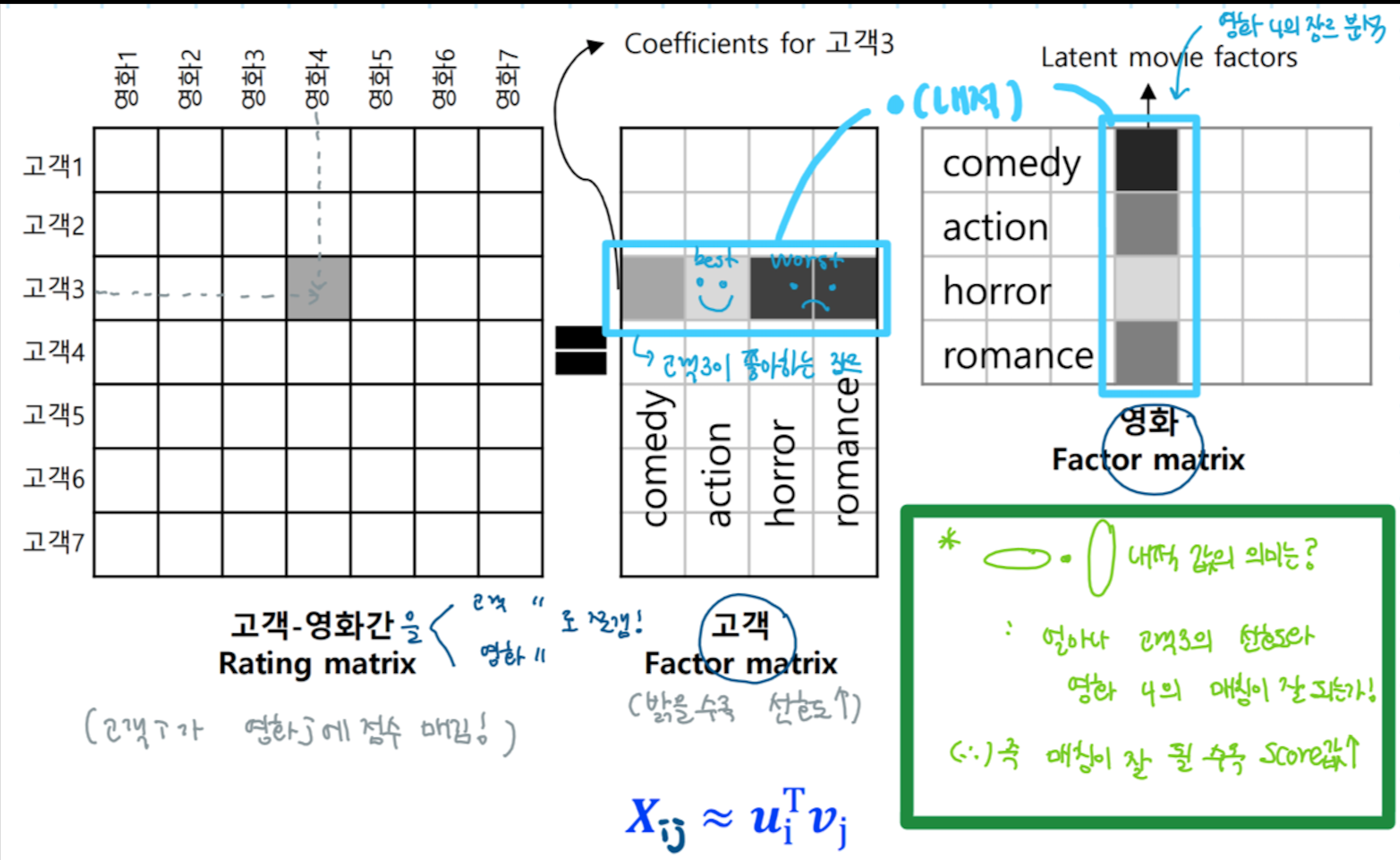
Collaborative prediction for recommendation(활용 예1)
추천 서비스 알고리즘 예시 <고객들의 영화 선호도>
0.3 Data covariance matrix
1) Data Covariance matrix
: data 분포(data 변수들간의 상관관계(분산) 표현)를 NxN matrix로 표현한 것.
예시 : apple & banana preference : 사람들의 사과/바나나 선호도 조사 -> 두 선호도 사이의 상관관계를 분석하는 것이 목표!
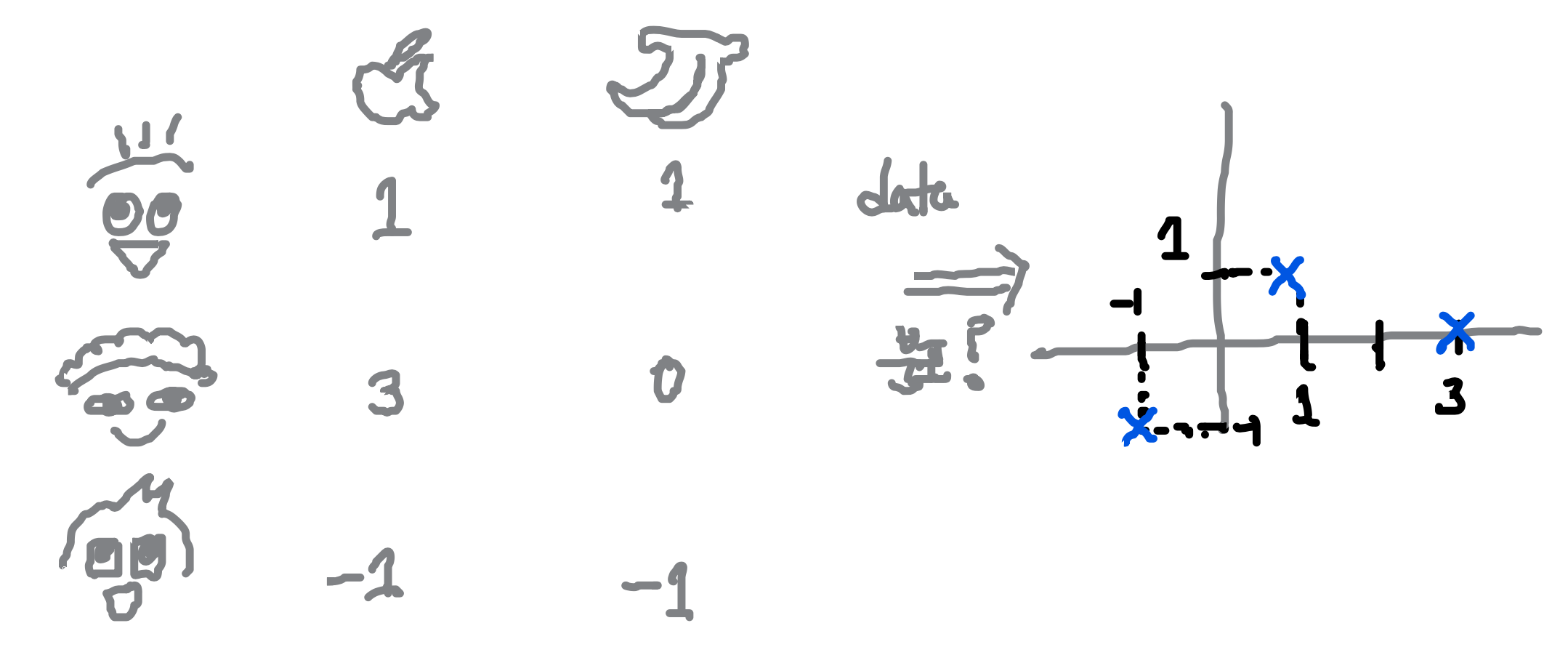
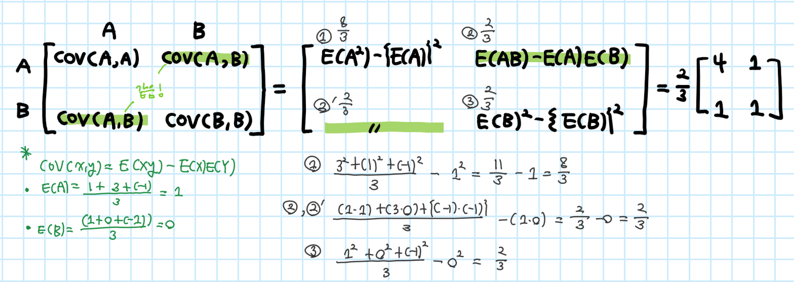
2) Covariance matrix 계산
1. Determinant & trace
1.1 Determinant
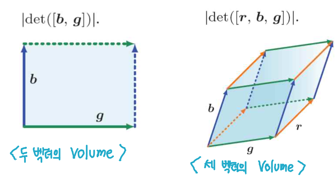
정방행렬 A(NxN)의 determinant는 column vector에 의해 확장(span)된 평행사변형(parallelogram)의 부피에 해당하는 실수에 A를 매핑하는 함수이다 ( det(A) 혹은 |A|에 의해 나타내짐)
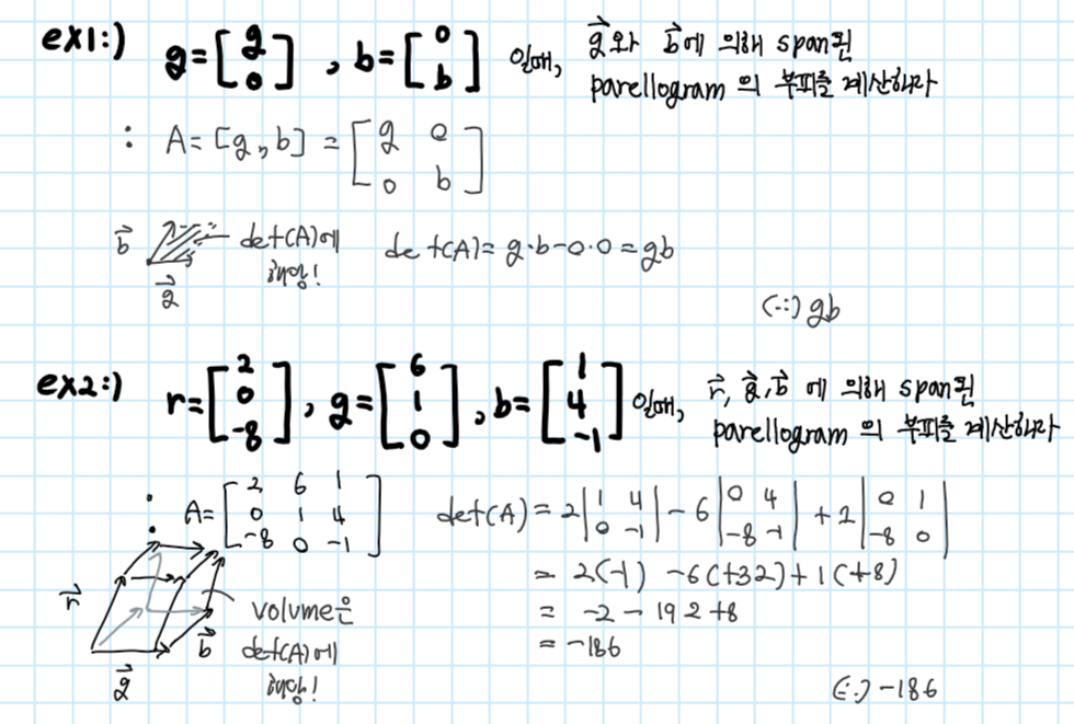
예시1),2)
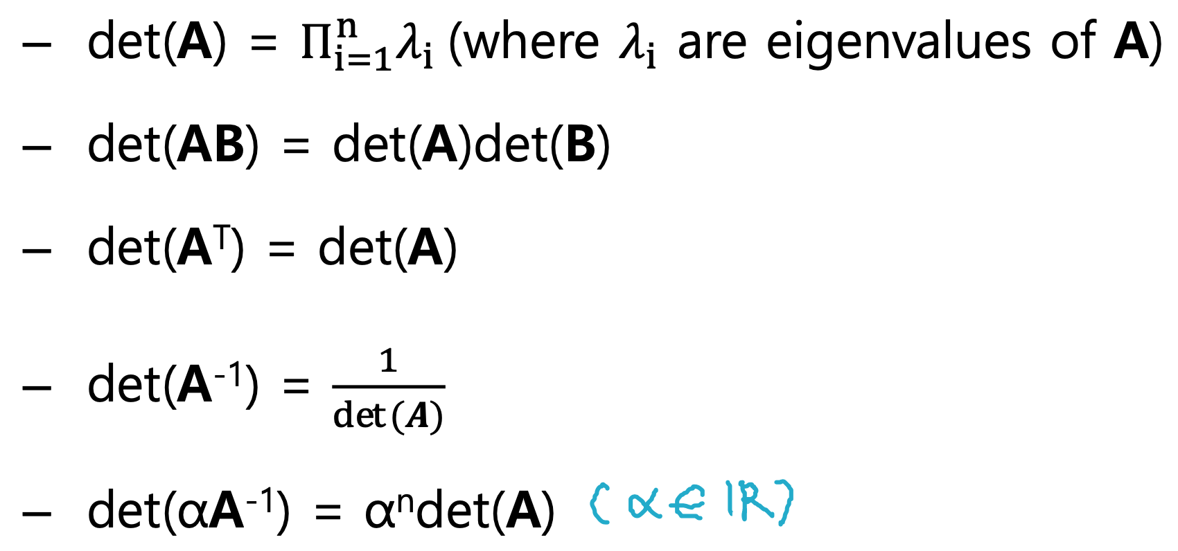
1.2 Properties of determinant
필요시 마다 아래 det에 대한 특징 참고
이론1.
정방행렬 A(NxN)의 determinant가 0이 아닐 경우 가역행렬 A^-1를 구할 수 있다
이론2.
정방행렬 A(NxN)의 determinant가 0이 아닐 경우 행렬 A는 full rank이다. (rank(A) = n)
* full rank란? linearly independet A의 column vector의 최대 개수에 해당
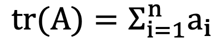
1.3 Trace(대각합)
Definition
: trace란 대각합으로 정방행렬 A(NxN)의 대각합을 말함
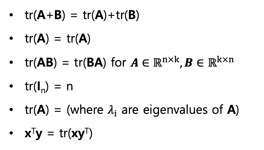
대각합의 성질
*마지막 대각합 성질 예시
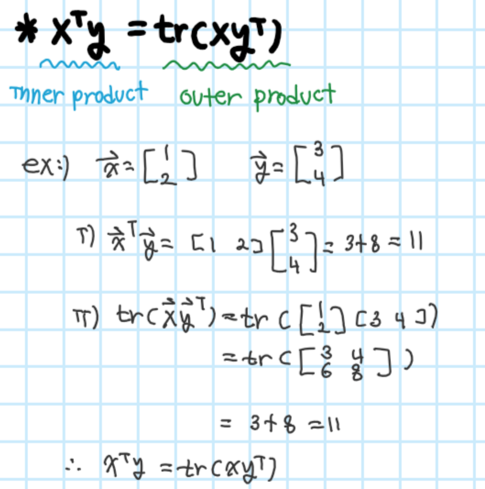
예시
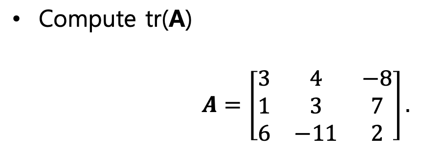
tr(A) = 3 + 3 + 2 = 8
2. Cholesky decomposition
Definition
matrix A가 symmetric하고 positive-definite(x^tAx > 0)인 경우에는 cholesky decomposition을 사용해 더 numerically stable하고 빠른 연산을 할 수 있다.
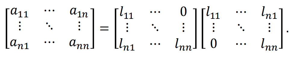
cholesky decomposition은 아래와 같이 행렬 A를 lower trianglular matrix L을 이용해 나타낼 수 있다.
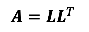
단, L은 Positive diagonal element를 가지고 있다
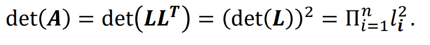
이 성질을 이용할 경우 아래와 같이 determinant를 효율적으로 계산할 수 있다
<성질 참고>
det(L^t) = det(L)
det(LL^t) = det(L)det(L^t) = (det(L))^2
cholesky decomposition & linear equation
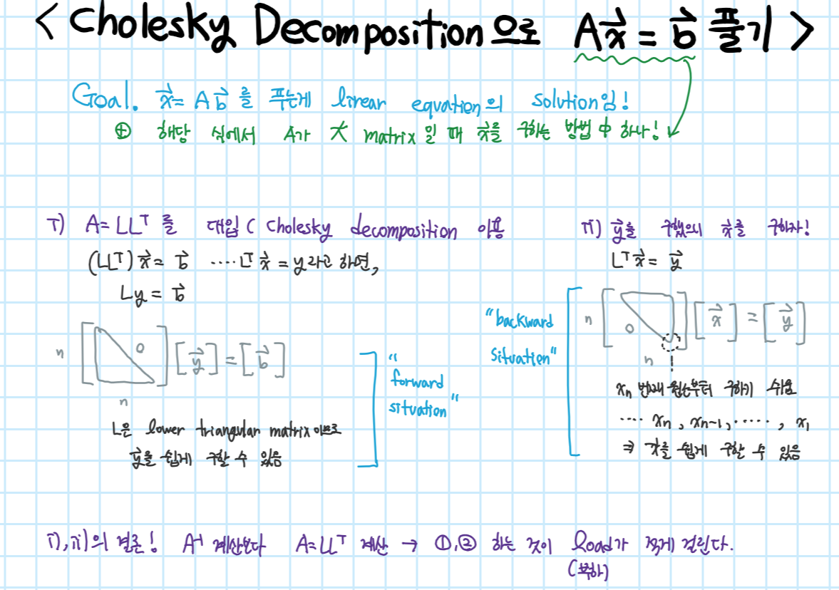
- cholesky decomposition 방법으로 구현시 linear equation에서 계산량 측면에서 이득을 봄
3. Eigendecomposition: Eigenvalues & eigenvectors
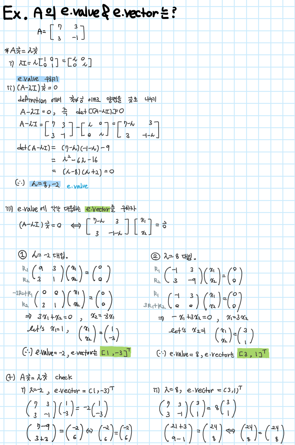
3.1 Eigenvalues & eigenvectors
Definition
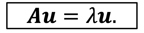
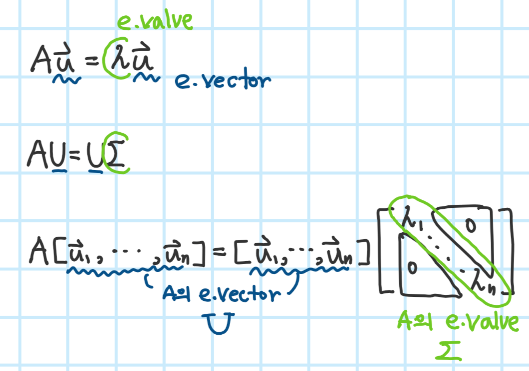
A를 nxn 정방향 행령이라고 하고, A의 eigenvalue를 λ, A의 eigenvector를 u라고 하면 다음과 같은 식이 성립한다
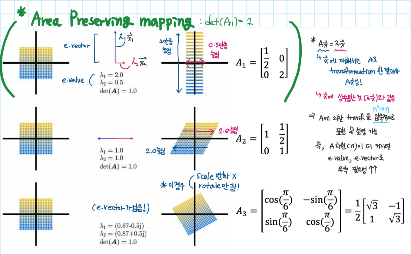
해당 식의 기하학적 의미
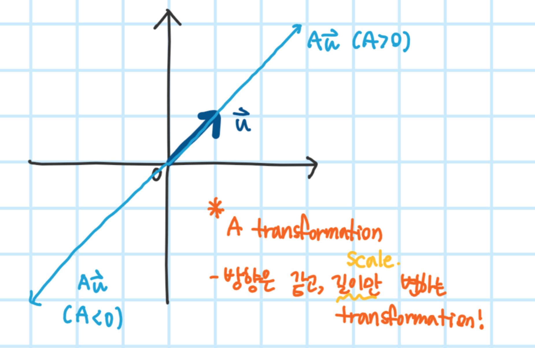
*주의. e.vector는 유일하지 않음, 단 vector의 비율이 같은 쌍들이 존재(보통 길이가 1인 e.vector 사용)
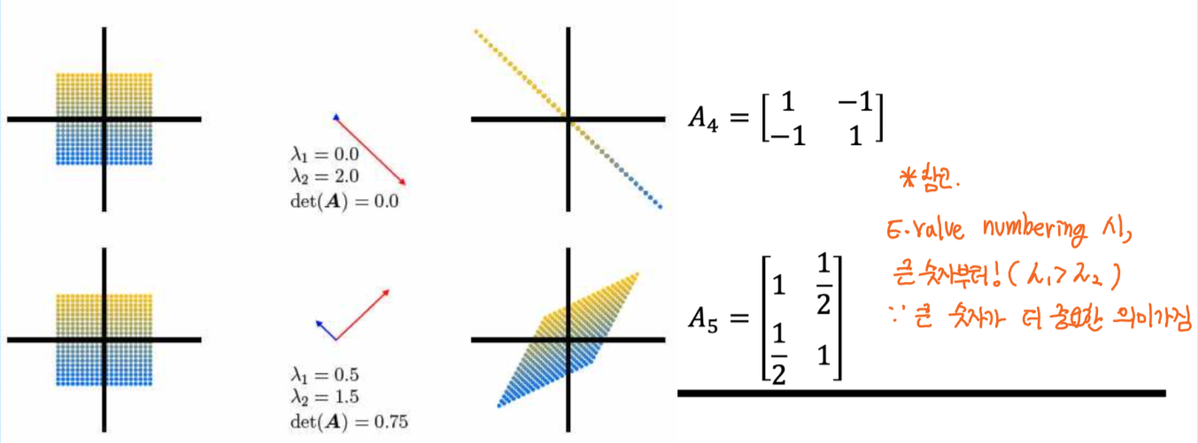
Graphical intution in 2D
transformation by five matrices
3.2 Eigendecomposition
3.2.1 Spectral decomposition
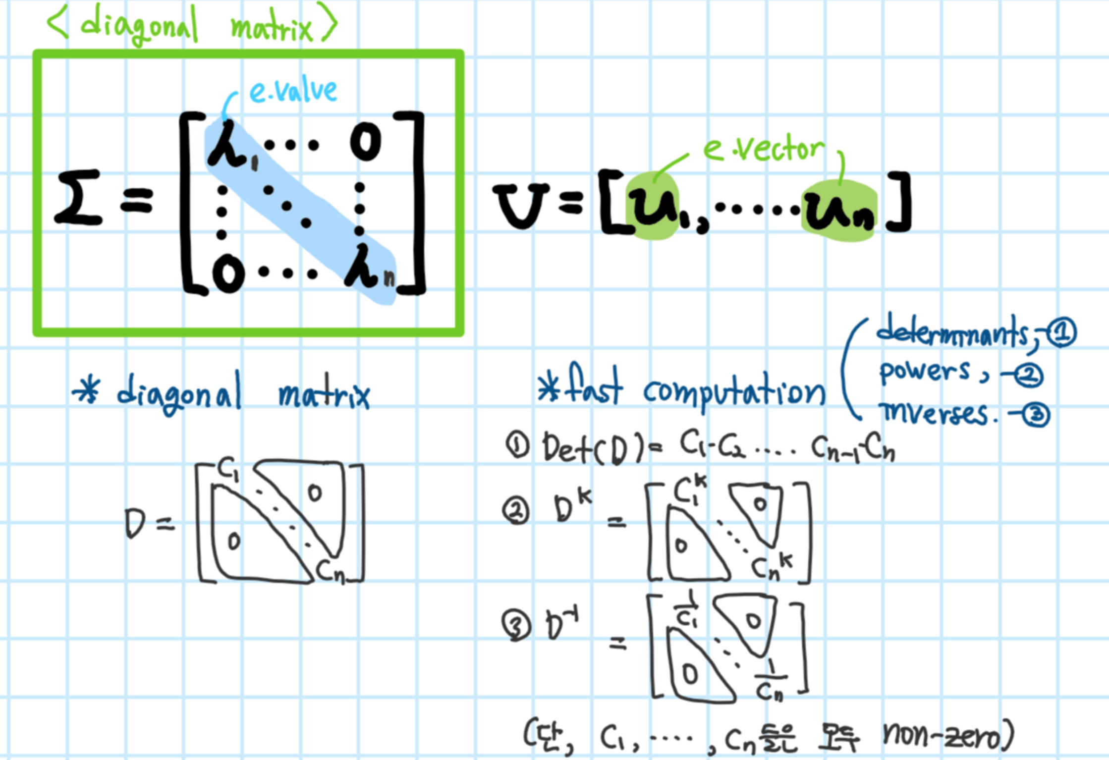
Definition(Diagonalizable)

diagnoal matrix의 장점
빠른 계산 속도
1. determinants
2. powers
3. inverses
*단, A는 diagonal matrix가 아닌 diagonalizable한 행렬임!
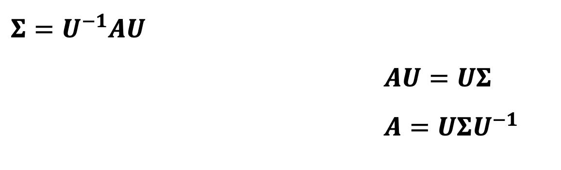
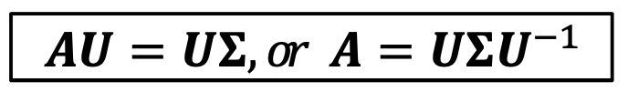
A의 n개의 e.vector가 linearly independent(선형 독립)하다고 하자. 이 경우 아래와 같은 식이 성립하고,
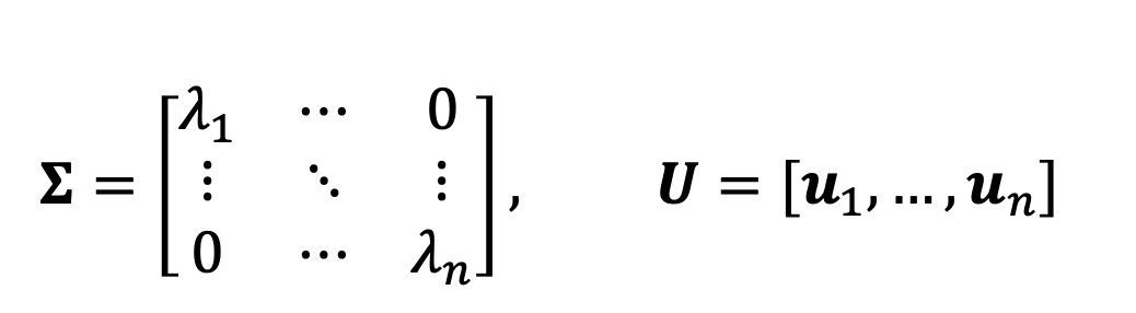
이는 아래의 식을 도출해낼 수 있다
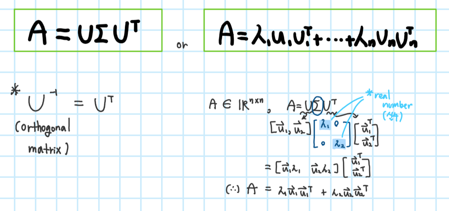
3.2.2 Eigendecomposition for symmetric matrices
Theorem(Spectral theorem)
정방향 행렬 A가 Symmetric하다면 e.value는 모두 real number이며 e.vector인 {u_1, ..., u_n}이 orthonormal하다
*orthonormal이란? 벡터들이 서로 orthogonal(independet 함)하면서 길이가 1인경우
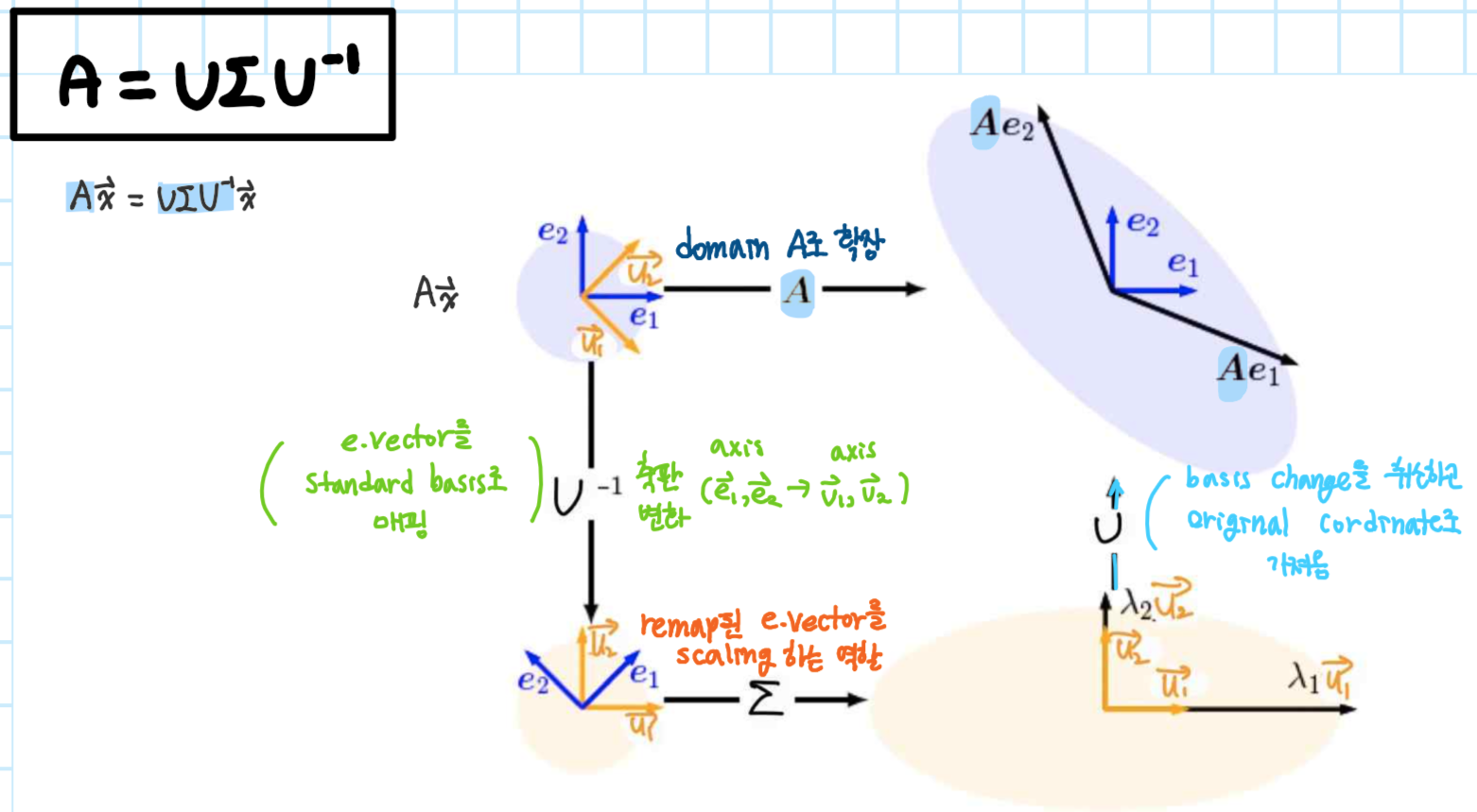
Geometric intuition for the eigendecomposition
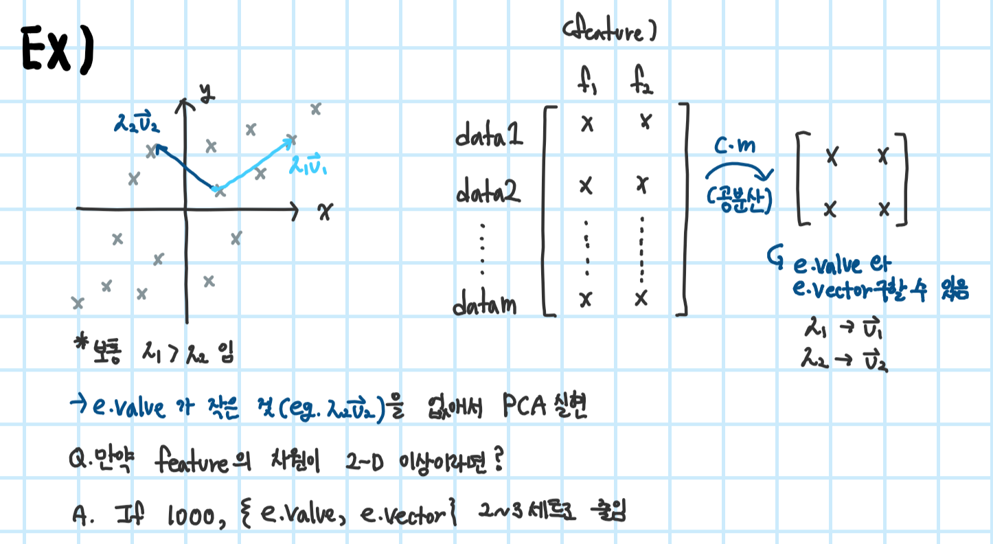
Intuition between eigendecomposition & PCA
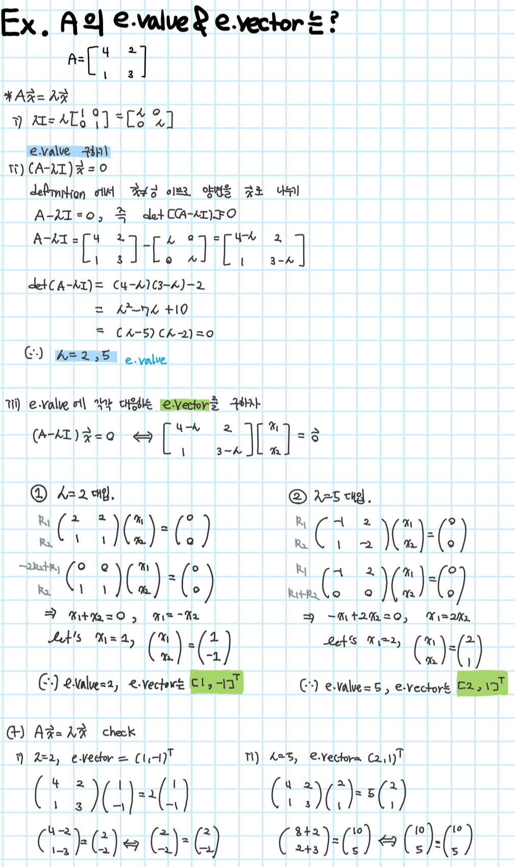
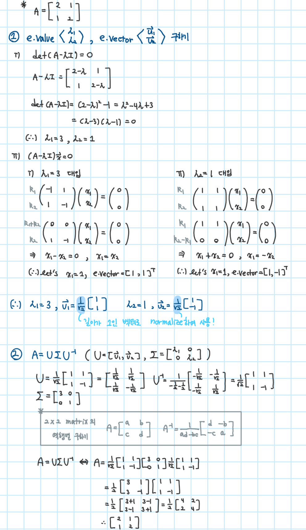
Example) Compute the eigendecomposition of A
+ Matrix decomposition & representation learning
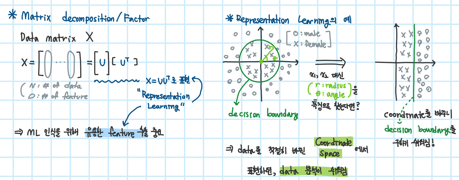
Representation Learning?
Why representation learning?
Matrix decomposition & representation learning
- RL 관점에서 matrix decomposition은 방법 중 하나이다 ( X = UU^T)
- "Latent Structure"은 matrix factor를 찾아 좋은 representation으로 data 분석을 쉽게 해준다
- RL은 머신러닝 주요 분야 중 하나로 크게 두가지로 나뉜다
1. 지금 배운 matrix decomposition
2. 이후 배울 SVD
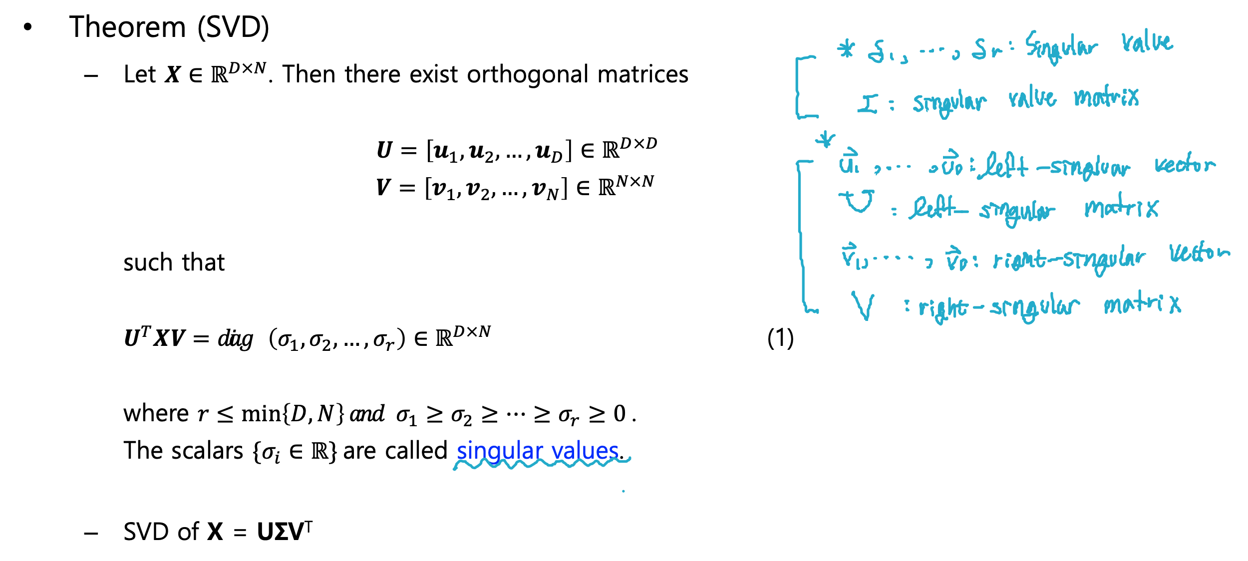
4. Singular value decomposition (SVD)
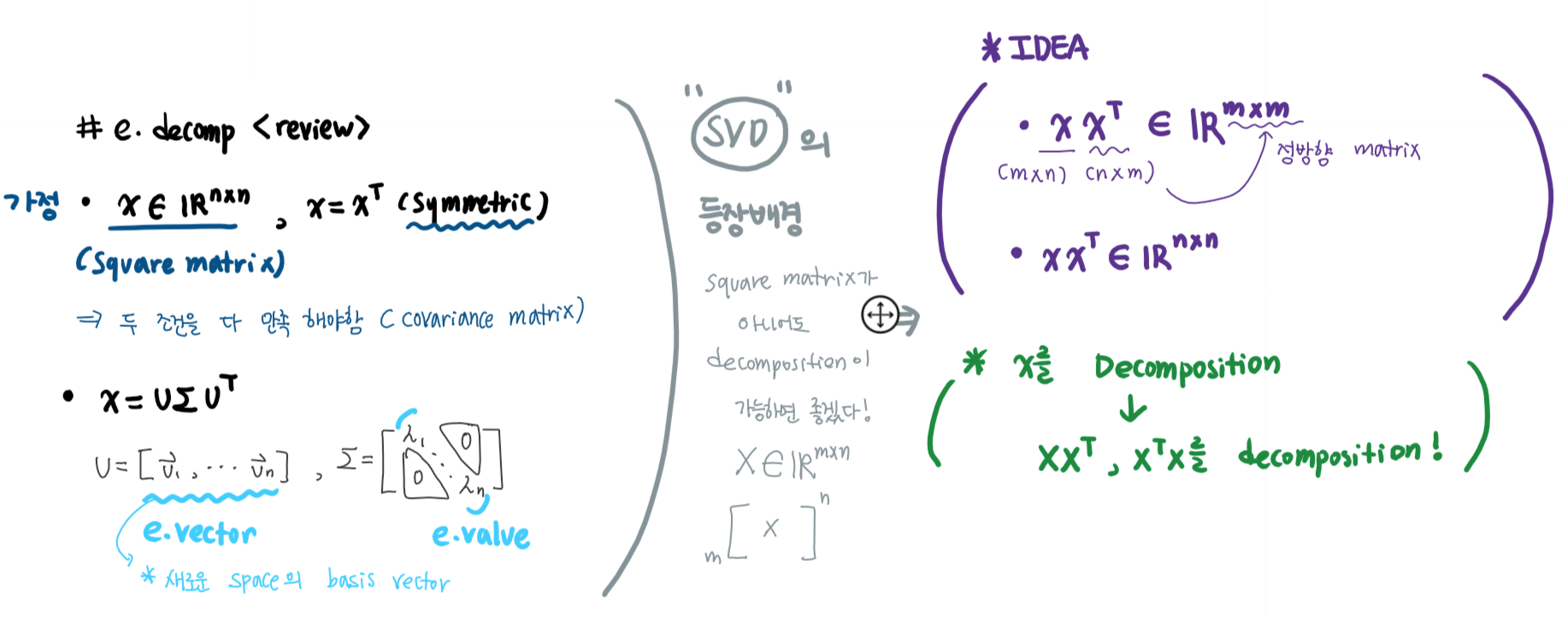
(Review) eigendecomposition
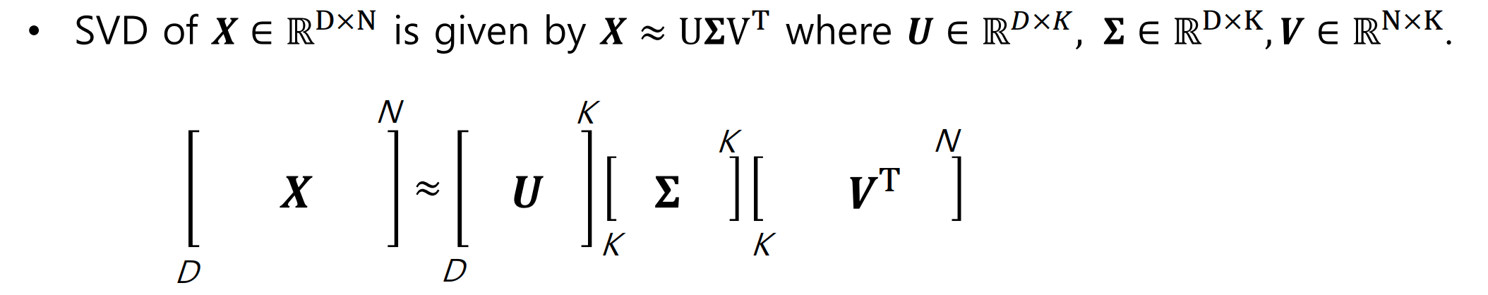
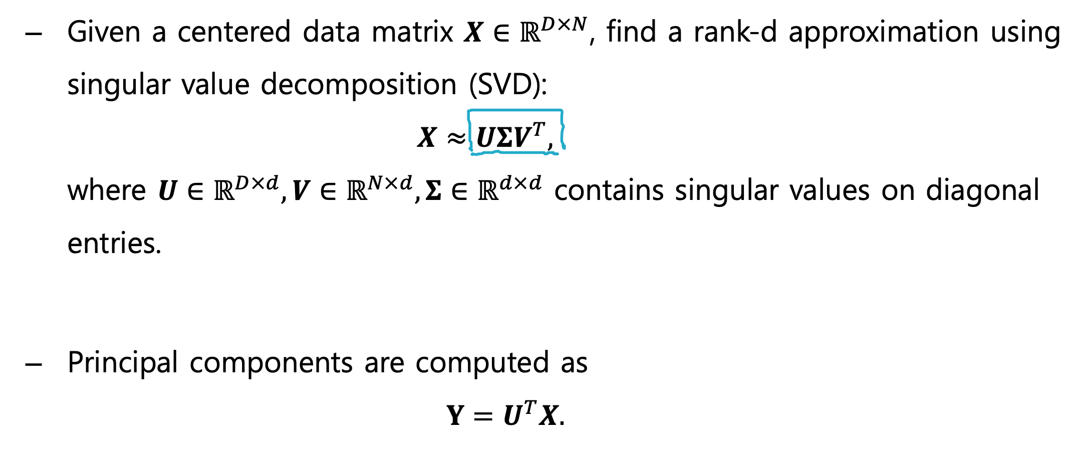
Idea of SVD & SVD
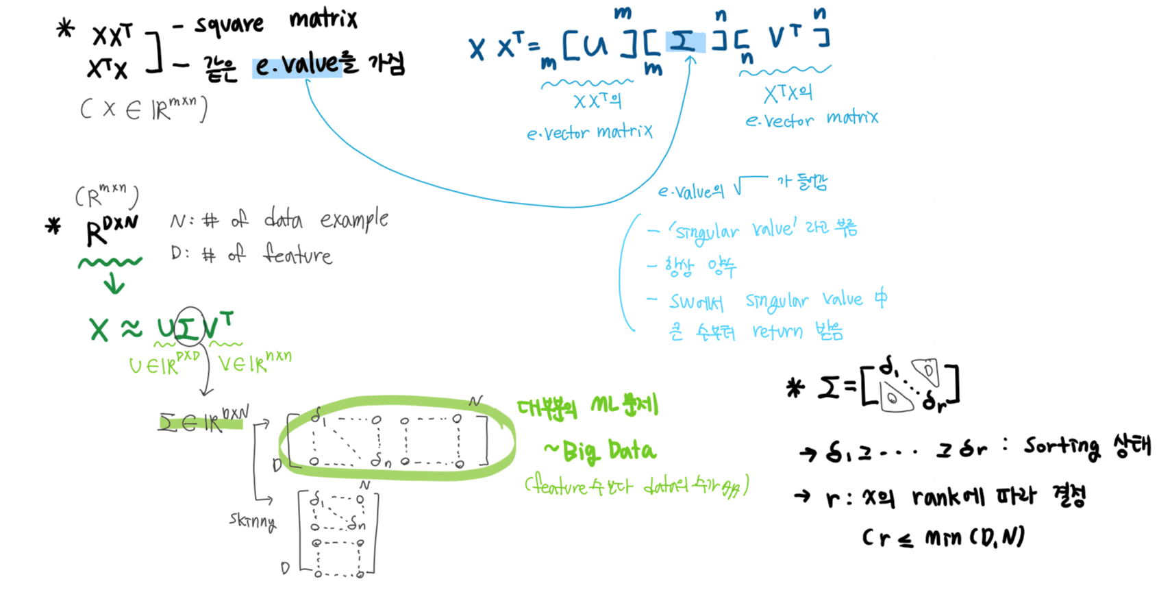
- Σ는 대각성분으로 singular value를 가지고 있으며, singular value matrix라 부른다
- 행과 열이 다른 matrix에 대한 decomposition을 수행할 수 있다는 장점이 있따
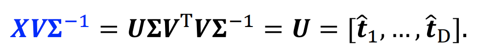
- XX^T, X^TX는 같은 eigenvalue를 가진다
- U는 XX^T eigenvector matrix이며, X에 대한 SVD의 left-singular matrix라 한다.
4.1 Alternatively by SVD : PASS
4.2 Singular value decomposition (SVD) : PASS
Movie ratings & its SVD(3 people, 4 movies)
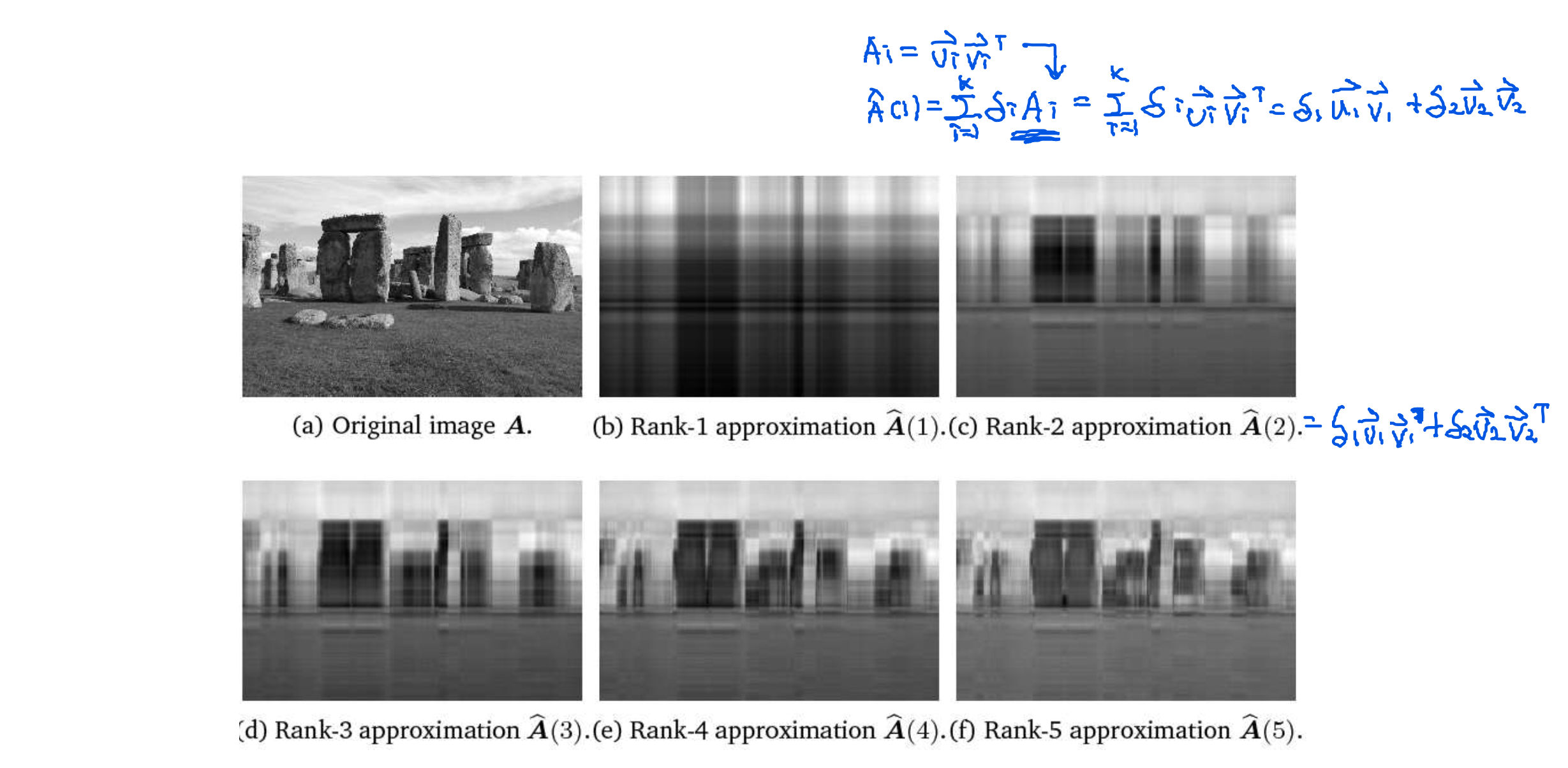
4.3 Low-rank approximation
Low-rank approximation의 용도
1. Representation learning 으로써, 영상의 중요 latent vector 를 구하는 데 사용될 수 있다.
2. 이미지 전송량을 줄이는 데 사용될 수 있다.
3. Full rank approximation으로 원본 영상을 복원할 수 있다
4. 미리보기 영상을 위해 영상을 요약하는 용도로 사용될 수 있다.
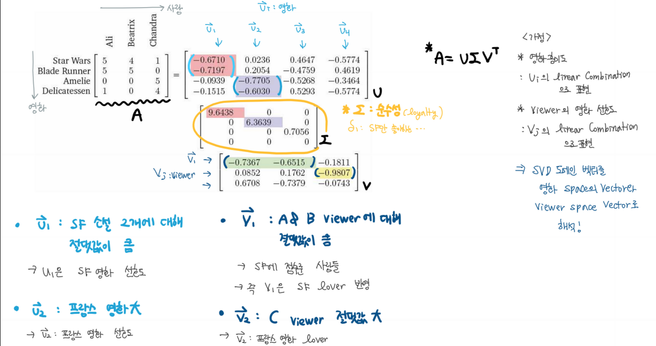
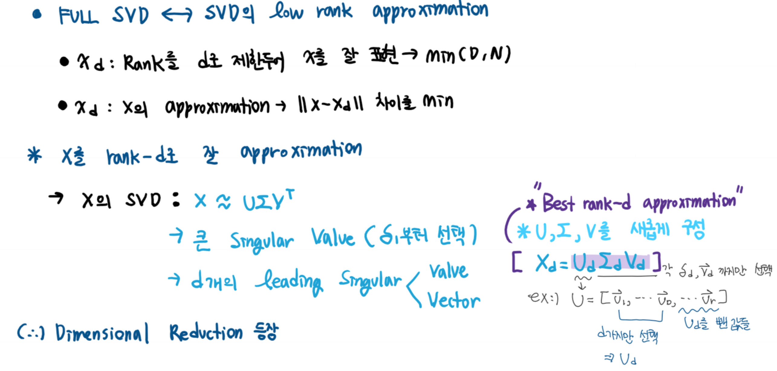
Image Processing with the SVD
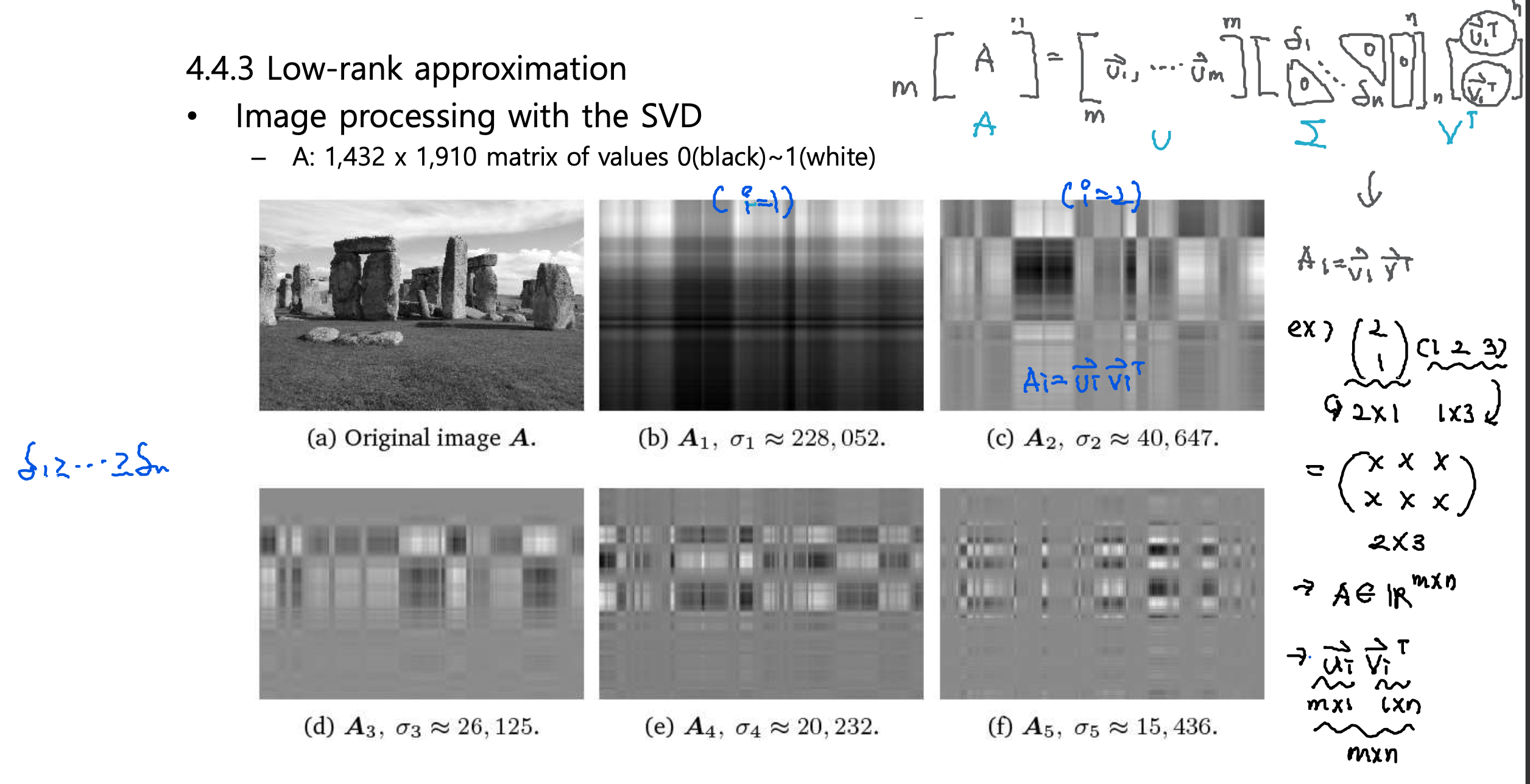
Image reconstruction with the SVD
'인공지능(AI) > 인공지능기초수학' 카테고리의 다른 글
| 05 Probability (0) | 2020.12.17 |
|---|---|
| 03 Analytic Geometry (0) | 2020.10.20 |
| 02 Linear Algebra (0) | 2020.10.18 |
| 01 Introduction AI Basic: 인공지능, 기계학습이란? (0) | 2020.10.18 |
| 00 인공지능 발전사 (0) | 2020.10.18 |